Fargo Ratings are ELO-like ratings for pool.

But there's more to the story. This is a description of what ELO ratings are, what FargoRate does, and how these are related. Nothing here is necessary to have a good functional understanding of Fargo Ratings and how they work. But for those who are interested, this is a peek behind the curtain.

The phrase ELO-like refers to any of a wide variety of schemes to rate competitors in activities that involve relative performance. They are named for Arpad Elo, a physics professor at Marquette University in Milwaukee who applied the ideas to chess a half century ago. So the ratings could be for pool, for chess, for arm wrestling, for tennis, for staring contests, for the game of chicken, for various online video games, for soccer, for ping pong, for football, or for any of a host of other activities.

This is to be distinguished from activities that involve absolute performance, like golf, bowling, weightlifting, running, and jumping. These don’t need an elaborate rating scheme: if Bubba in New Orleans long jumps 7.7 meters, and Vlad in Moscow jumps 7.9 meters, Vlad is better.

I describe here as clearly as I can first what is common to all the ELO-like rating approaches. Then I describe the implementation of the basic ELO scheme that FIDE (international chess organization) uses. FIDE’s approach, if not the gold standard, has history on its side. And it is the easiest to understand and implement. I follow this by a brief description of improvements to the FIDE approach (what we refer to as the Old Fargo Rating approach as well as other schemes like the Glicko approaches in chess). Finally I describe something quite different: what FargoRate actually does.

What is the same about all these ratings schemes?

The basic feature common to all ELO-like approaches is this:

A’s chance beating B depends only on the rating difference between A and B.

That indented, bold, italic statement is it. Nothing else needs to be said.

Where’s the Math?

Believe it or not, though, that simple statement says more than it seems like it says and actually has mathematics in it. The indented, bold, italic statement forces a particular kind of relation between rating difference and chance of each player winning, namely, a player’s chance of winning must follow something raised to the POWER of the rating difference.

chance of winning ~ (##)^(rating difference)

Here "^" means raiseed-to-the-power-of. Nothing else will work. No other choice is consistent with the indented, bold, italic statement.

One way to see the mathematics in this statement is to recognize the phrase “depends only on” can be turned into “=” once the particular dependence is expressed. So “chance” is on one side of the equation and “rating difference” is on the other side. The phrase “chance” refers to, for example, player A’s wins divided by the total number of games or similarly player A’s wins divided player B’s wins. Importantly it is a ratio involving players A and B. The right hand side is a difference involving players A and B. Anytime multiplication or division happens on one side of an equation and addition or subtraction happens on the other side, there is no choice but to find the above form, or, equivalently, that the rating difference is related to the logarithm of the chance

Logarithm(chance) ~ rating difference

The important point here is that any equations that relate chance or expectation to rating difference do not come from a vacuum. Other than an arbitrary choice of the size of a rating point, the relations are forced by the indented, bold, italic statement.

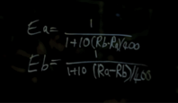
For Fargo Ratings, two players will win games in the ratio,

ratio = 2^(rating difference/100)

For many of the other schemes, players will win in the ratio,

ratio = 10^(rating difference/400)

The distinctions between these (note the 2 versus the 10 and the 100 versus the 400) are inconsequential and are just a matter of taste. Both these relations, once again, are just a restatement of the indented, bold, italic sentence above. They add nothing to it. What this means is if you have accurate ratings—the all elusive true ratings--for two players for any of these activities, you can calculate the chance of each player winning the next game.

Algorithm?

The Mark Zuckerberg character In the Facebook movie (Social Network) says to his friend, Eduardo, with some urgency in his voice,

“ I need the algorithm you use to rank chess players…
We’re ranking girls…
I need the algorithm
I need the algorithm…”
And Eduardo writes this on the dormitory window:

Note the similarity with the expressions above, the 10^(rating difference/400). The problem, though, is that as cool as it sounds in the movie, this relation is not an algorithm and is nothing more than a restatement of the underlined sentence.

An algorithm is a set of instructions, something you might program a computer to execute. If the subject is home-baked cookies, the algorithm is the recipe. The above, by contrast, is at best a cookie. And it only tastes good if the ratings are accurate. Calculating the chance of each player winning from the ratings—like eating the cookie-- is the easy part. Getting the ratings is the hard part. These equations say nothing about how to get the ratings.

A Sad Truth

Before discussing different rating approaches, we must acknowledge a sad truth. The ratings in Eduardo’s scribble? We don’t know them and never will. Yes, every participant has a true rating-one that we might imagine is tattooed to the inside to the participant’s chest where we can’t see it. The participant also has a tentative rating, one that perhaps is written on an erasable sign he hangs around his neck.

The usual approach to getting the ratings goes something like this. Start with a guess for everybody’s rating—maybe everybody starts at the same number or maybe you use some other criteria to make an educated guess. These initial ratings are highly tentative, and the goal is to be informed by actual game results to make them better. Even when they get better, and even when they get a lot better, our best current ratings are always tentative and are open to being informed by even more actual results. They are still the ones written on the sign around the player’s neck and not the ones tattooed to the inside of the player’s chest.

What’s different about the rating schemes?

Exploring a particular example of a rating update helps to illustrate the difference between the common approaches. In our example, two players are going to play 10 games. Their current ratings—the tentative ones we work with-- lead to an expectation of how many games each player will win. This is easy to calculate. Suppose Player A is rated 575 and B is 525. The first thing to do is compute a transformed version of the ratings to make life easier. A’s transformed rating is 2^(575/100). We’ll call that TA. B’s transformed rating, TB, is 2^(525/100). These two players are expected to win games in the ratio TA/TB.

It is that simple.

So for 10 games, player A is expected to win EA = 5.9 games, where

EA = (TA/(TA + TB)) * 10.

Player B is expected to win EB =4.1 games.

Now the match happens and the actual score is 7 to 3. So player A exceeded his or her expectation by 1.1 games (7.0 - 5.9). And player B fell short of his or her expectation by 1.1 games.

A’s rating should go up and B’s rating should go down. And it makes sense the amount they go up and down should be higher if the actual results differed more from the expectation. So we propose

Player A’s rating change = K * (1.1)

Player B’s rating change = K’ * (-1.1)

The big problem is these new factors K and K’ just appeared. So you want to increase A’s rating. But by how much? You have to make a choice for K. If you choose K too small, then ratings adjust very slowly and are too stable. If you choose it too big, then you will overshoot and the ratings will tend to bounce around too much.

There has been a lot futzing around about what to use for K. Maybe you analyze historical data to help you out; Maybe K is different for higher and lower rated players; Maybe K depends on how many previous games each player has played, and so forth. Most implementations of ELO schemes differ by how they choose K and what it depends upon. FIDE, the international chess organization, has probably the most celebrated implementation of an ELO rating scheme, and they use a rather unsophisticated choice for K.

Here is an excerpt from the FIDE website.

8.56
K is the development coefficient.
K = 40 for a player new to the rating list until he has completed events with at least 30 games
K = 20 as long as a player's rating remains under 2400.
K = 10 once a player's published rating has reached 2400 and remains at that level subsequently, even if the rating drops below 2400.
K = 40 for all players until their 18th birthday, as long as their rating remains under 2300.

So FIDE is just guessing.

Old Fargo Ratings

When we derived, back in 2002, the maximum likelihood approach described later, one of the byproducts of our efforts was a theoretical estimate for a sensible K value. In particular, if A and B play 10 games, then the K value for A is

K = 630 * (RB-10)/(RA*RB).

Here RA and RB are the robustness values (total number of games, including current and previous games) for A and B. Note some interesting things about this K value. First, suppose a player’s opponent is a complete unknown. Intuitively the first player’s rating shouldn’t be affected by winning or losing against an opponent for whom we have no information. Sure enough, in this case RB=10 and this makes K equal to zero. Likewise, if the opponent is poorly established, K will be smaller. And finally if the first player himself is well established, K will be smaller.

The simple ELO update with the above value for K is what we did for years before we began doing the ab initio global optimization (described below) in late 2014.

Mark Glickman has developed improved approaches for chess (Glicko and Glicko-2 systems) that similarly choose sensible values for K that take into account how well established are a player’s and the player’s opponent’s ratings.

Old Fargo and Glicko are improvements on the simple ELO scheme that FIDE uses, and FIDE should be using something better. Likely they are not because,

• reluctance to lose the feature that players can simply compute their own rating change (transparency)
• not wanting an angry mob of grand-master chess players who lost a spot or two on the ranking list
• politics

FargoRate: A Different Direction

In principle, using the above schemes, player ratings will eventually get to a reasonable estimate of the true rating that forgets the particular choice of the starting guess and that is independent of the particular choice for K. This is true provided everybody plays a very large number of games and the choice for K is sensible. In practice, though, many players in the system don’t play a large number of games, and the starter-rating choice lingers. This is a particularly vexing problem with two nearly isolated groups, one of which is rated too high relative to the other.

A player’s true rating—the one we don’t have—drifts in time as the player’s skill improves or deteriorates. That player’s tentative rating—the one we do have--also changes in time due to skill changes. But the much bigger reason the tentative rating changes in time is that more data is moving the tentative rating closer to the elusive true rating.

With this in mind, imagine we either ignore the slow drifting of true skill or we limit ourselves to games played during a period of time sufficiently short that we can safely ignore actual skill changes.

Now rather than using a sequential update scheme like all of the above, we imagine we take our large number of players and assume nothing about them. Then we take our very large number of games that have been played amongst all these players and we imagine all those games are played out in front of us right now.

There exists a set of tentative ratings for every player in the system such that the matches—all the matches amongst all the players—turning out exactly like they did was most likely. This in the field of statistical inference is called the maximum likelihood approach.

Maximum Likelihood

Let’s start with a simple example of the maximum likelihood idea. Suppose a new player—Victor—moves to town and plays 20 games against Leroy, a well established player. The question is how does Victor play compared to Leroy? What is the rating difference between Victor and Leroy? Suppose each player wins 10 games. So the score after 20 games is 10 to 10. It seems reasonable to suggest they play about the same—have the same rating.

But of course this doesn’t have to be the case. What is it about that intuitive choice that makes it better than other choices? How can we justify the tentative proposal that these players have the same rating over alternative proposals?

Here are some possibilities that can be true even with the 10-to-10 game history.

A. Victor is a much better player than Leroy
B. Victor is a somewhat better player than Leroy
C. Victor and Leroy play the same
D. Victor is a somewhat weaker player than Leroy
E. Victor is a much weaker player than Leroy

If A is true, then Victor had an unusually poor day or Leroy had an unusually good day for the 20 games or both. That is, given A, the actual results are possible but pretty unlikely. Likewise, given D, the actual results are somewhat unlikely. And given C, the actual results are somewhat more likely. These likelihoods form a curve that looks something like the following:

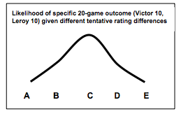
The maximum likelihood idea is we choose as our best tentative rating difference the one for which the actual results were most likely. So we choose C, that Victor plays at the same level as Leroy.

How does the situation change if Victor and Leroy played 200 games with a score of 100 to 100 instead of 20 games with a score of 10 to 10? Now possibilities A and E are extremely unlikely, and possibilities B and D are more unlikely than before. The curve looks more like the following:

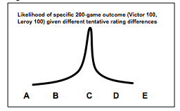
So after 200 games, the likelihood is more peaked at the maximum and we are more confident our tentative rating difference is closer to the true rating difference.

The left-right direction in the curves of the above two figures is the rating difference, and the up direction is the likelihood. If we add a third player, then there are two rating differences. One can be left-right and the other front-back. The up direction is still the likelihood.

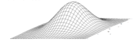So instead of a likelihood curve, we have a likelihood surface. Our best tentative ratings are the ones that reflect the top of the mountain.

With thousands of players there are thousands of “directions.” We can’t display it with a plot, but the surface becomes a many-dimensional hypersurface, and the concept of a likelihood mountaintop is still valid. Once again, our best tentative ratings are the ones for which the actual game results –all of them—turning out the way they did is most likely.

Locating the top of the mountain is not easy, but it is a well defined mathematical problem. Each day, as new games are added to the system, the detailed shape of the mountain shifts. As more data is added for the same group of players, the mountain generally becomes more peaked. Importantly though, the location of the peak also shifts, and this means optimum ratings for the players shift with the new data.

In general, the mountain is sharply peaked in some directions and relatively flat in others, and the curvatures in different directions give us information about variances and covariances—about how confident we are in a particular player’s rating and how sensitive is one player’s rating to another player’s rating. In fact we can compute, at the mountain peak, something called the Fisher Information Matrix that has this curvature information. But in any case the optimum ratings are what they are. They don’t depend on the details of the path or approach we take in climbing the mountain.

Every day, FargoRate constructs the mountain for all the available game data amongst all the players. Current games are given full weight, and there is an exponential decay of the weight of past games such that 3-year-old games contribute half, 6-year-old games contribute a quarter, and so forth. This time decay helps account for actual skill changes Every day the mountain is scaled to determine the optimum ratings.

We refer to this process as ab initio global optimization. The Latin phrase ab initio means from the beginning, or from first principles.

Sisyphus has it easy

As I write Sisyphus is rolling his big boulder up the hill as he will do for eternity only to have it roll down to where he must start over again. Like Sisyphus, FargoRate must scale the mountain every day. But unlike Sisyphus, FargoRate must begin by actually constructing the day’s mountain.